The IS Curve and Aggregate Demand
Week 04
March 2, 2026
Financial Frictions and Investment
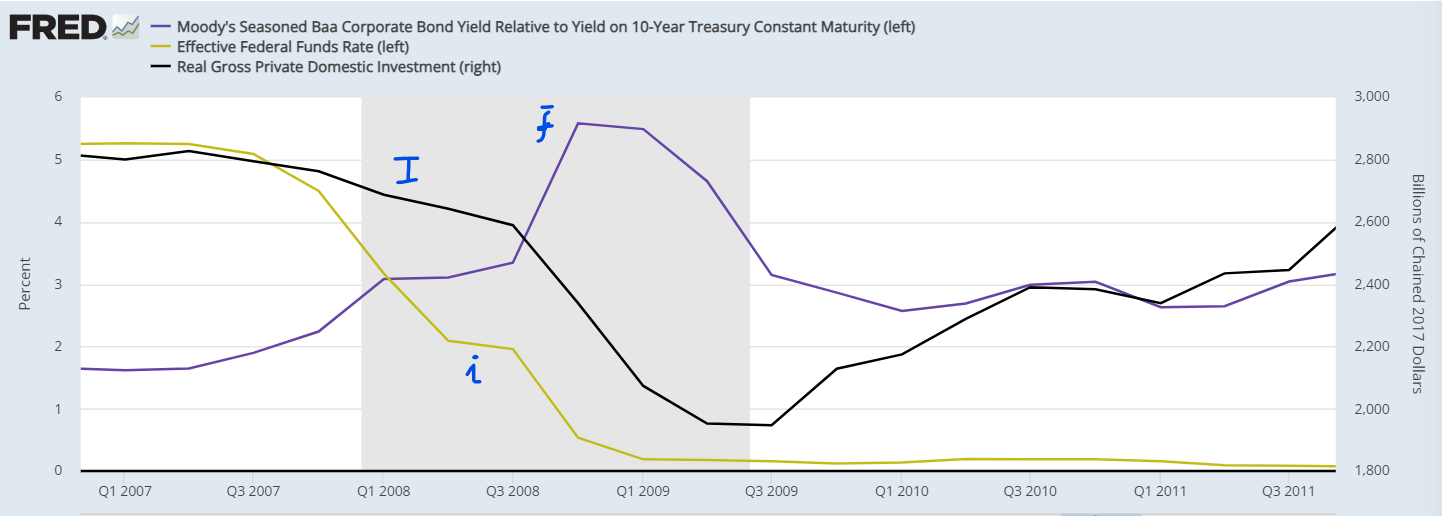
In the great financial crisis of 2007-2010, the inverse relationship between \((\overline{f})\) and \(I\) can be easily spotted in the figure below: \(\uparrow \overline{f}, \downarrow I\), despite \((i)\) going down. And \(\downarrow \overline{f}, \uparrow I\), despite \(i\) remaining at \(0 \%\).
IS Curve: Graphical Representation
For a given level of \((\overline{A})\), an increase in \((r)\) will cause a reduction in aggregate demand \((D)\), which will lead to a decline in GDP \((Y)\), and vice-versa. 
IS Curve: Graphical Representation
- \(\Delta r=+2pp\)
- \(\Delta \overline{A}=0\)
- \(\Delta Y=-2 trillion\)
- If \(\Delta \overline{A} \neq 0\), the IS would shift to the right/left
A Shift in the IS: a Graphical Example
If \(\uparrow \overline{G} \ \Rightarrow \ \uparrow \ \overline{A} \ \Rightarrow \ \uparrow Y\) , the IS shifts to the right:
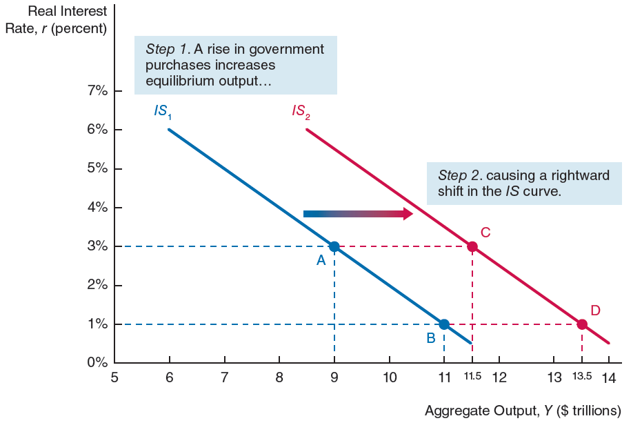
- The IS shifts to the right for any \(r\) level
- The shift is the same for \(r=3\%\), \(r=1\%\), \(r=0\%\) , or …
A Shift in the IS: another Graphical Example
If \(\uparrow \overline{T} \ \Rightarrow \ \downarrow \ \overline{A} \ \Rightarrow \ \downarrow Y\), the IS shifts to the left:
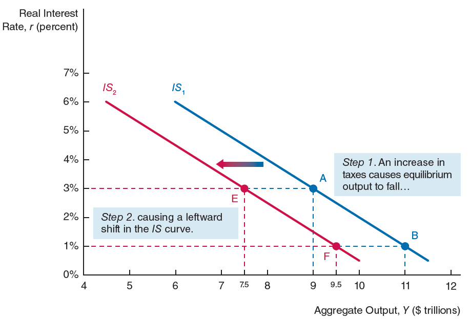
- The IS shifts to the left for any \(r\) level
- The shift is the same for \(r=3\%\), \(r=1\%\), \(r=0\%\) , or …
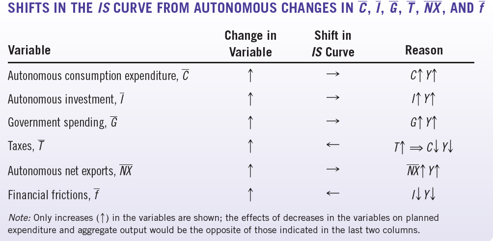
A Textbook Useful Table